Chapter 7

Chapter 7 of R4DS teaches how to import a variety of file types into R. This page will work through a subset of the chapter’s prompts. I’ll start by loading the tidyverse and a variety of packages to help us read different file types.

pacman::p_load(readxl, readr, tidyverse)

7.2.3 Exercises:

Exercise 7.2.3.1

What function would you use to read a file where fields were separated with “|”?

1 answer: this can be done with read_delim(). Firsts, let’s use the sales files in this chapter to create a spreadsheet with fields separated by “|”. Then we can read this file in R using the read_delim() function.

sales_files <- c(
  "https://pos.it/r4ds-01-sales",
  "https://pos.it/r4ds-02-sales",
  "https://pos.it/r4ds-03-sales"
)

sales <- read_csv(sales_files, id = "file", show_col_types = FALSE)

write_delim(sales, file = "./data/sales.csv", delim = "|")

sales_delim <- read_delim(
 "./data/sales.csv", delim = "|", show_col_types = FALSE)

sales_delim

# A tibble: 19 × 6
   file                         month     year brand  item     n
   <chr>                        <chr>    <dbl> <dbl> <dbl> <dbl>
 1 https://pos.it/r4ds-01-sales January   2019     1  1234     3
 2 https://pos.it/r4ds-01-sales January   2019     1  8721     9
 3 https://pos.it/r4ds-01-sales January   2019     1  1822     2
 4 https://pos.it/r4ds-01-sales January   2019     2  3333     1
 5 https://pos.it/r4ds-01-sales January   2019     2  2156     9
 6 https://pos.it/r4ds-01-sales January   2019     2  3987     6
 7 https://pos.it/r4ds-01-sales January   2019     2  3827     6
 8 https://pos.it/r4ds-02-sales February  2019     1  1234     8
 9 https://pos.it/r4ds-02-sales February  2019     1  8721     2
10 https://pos.it/r4ds-02-sales February  2019     1  1822     3
11 https://pos.it/r4ds-02-sales February  2019     2  3333     1
12 https://pos.it/r4ds-02-sales February  2019     2  2156     3
13 https://pos.it/r4ds-02-sales February  2019     2  3987     6
14 https://pos.it/r4ds-03-sales March     2019     1  1234     3
15 https://pos.it/r4ds-03-sales March     2019     1  3627     1
16 https://pos.it/r4ds-03-sales March     2019     1  8820     3
17 https://pos.it/r4ds-03-sales March     2019     2  7253     1
18 https://pos.it/r4ds-03-sales March     2019     2  8766     3
19 https://pos.it/r4ds-03-sales March     2019     2  8288     6

Exercise 7.2.3.2

Apart from file, skip, and comment, what other arguments do read_csv() and read_tsv() have in common?

2 answer: according to the help text, all arguments are the same between these two commands, such as col_names, col_types, col_select, ID, etc. We just use read_csv() vs read_tsv() when importing comma delimited files vs. tab delimited files, respectively.

#?read_csv
#?read_tsv

Exercise 7.2.3.3

What are the most important arguments to read_fwf()?

3 answer: the most important arguments include file and col_positions. col_positions specifies the width of the fields. Options are fwf_empty(), which guesses width based on the positions of empty columns; fwf_widths(), where you supply the width of columns; fwf_positions(), where you supply paired vectors of start and end positions; and fwf_cols(), where you supply named arguments of paired start and end positions/column widths.

#?read_fwf

Exercise 7.2.3.4

Sometimes strings in a CSV file contain commas. To prevent them from causing problems, they need to be surrounded by a quoting character, like ” or ’. By default, read_csv() assumes that the quoting character will be “. To read the following text into a data frame, what argument to read_csv() do you need to specify?

4 answer: utilize the quote argument

read_csv("x,y\n1,'a,b'", quote = "\'", show_col_types = FALSE)

# A tibble: 1 × 2
      x y    
  <dbl> <chr>
1     1 a,b

Exercise 7.2.3.5

Identify what is wrong with each of the following inline CSV files. What happens when you run the code?

5 answer: see each tab below

#original
suppressWarnings(
read_csv("a,b\n1,2,3\n4,5,6", show_col_types = FALSE)
)

# A tibble: 2 × 2
      a     b
  <dbl> <dbl>
1     1    23
2     4    56

#revision: there was one fewer column than needed; fix this by adding ", c" below
read_csv("a,b,c\n1,2,3\n4,5,6", show_col_types = FALSE)

# A tibble: 2 × 3
      a     b     c
  <dbl> <dbl> <dbl>
1     1     2     3
2     4     5     6

#original
suppressWarnings(
read_csv("a,b,c\n1,2\n1,2,3,4", show_col_types = FALSE)
)

# A tibble: 2 × 3
      a     b     c
  <dbl> <dbl> <dbl>
1     1     2    NA
2     1     2    34

#revision: there was one fewer column than needed; fix this by adding ", d" below. Also we can quiet a warning message by adding two commas after the first 2 to indicate missing values
read_csv("a,b,c,d \n1,2,,\n1,2,3,4", show_col_types = FALSE)

# A tibble: 2 × 4
      a     b     c     d
  <dbl> <dbl> <dbl> <dbl>
1     1     2    NA    NA
2     1     2     3     4

#original
read_csv("a,b\n\"1", show_col_types = FALSE)

# A tibble: 0 × 2
# ℹ 2 variables: a <chr>, b <chr>

#revision: add a backslash before last quote so that both quotes surrounding 1 have an escape; then add second quote after 1" to close the quotes for the entire string. Lastly, set quote argument equal to ""
read_csv("a,b\n\"1\",", quote = "", show_col_types = FALSE)

# A tibble: 1 × 2
  a       b    
  <chr>   <lgl>
1 "\"1\"" NA

#original
read_csv("a,b\n1,2\na,b", show_col_types = FALSE)

# A tibble: 2 × 2
  a     b    
  <chr> <chr>
1 1     2    
2 a     b

#revised: I'm unclear what the issue is that the authors are highlighting but my guess is that you likely don't need the 2nd row with values matching variable names
read_csv("a,b\n1,2", show_col_types = FALSE)

# A tibble: 1 × 2
      a     b
  <dbl> <dbl>
1     1     2

#original
read_csv("a;b\n1;3", show_col_types = FALSE)

# A tibble: 1 × 1
  `a;b`
  <chr>
1 1;3

#revised: use read_csv2 which is for files where fields are delimited with semicolons instead of commas
suppressMessages(
read_csv2("a;b\n1;3", show_col_types = FALSE)
)

# A tibble: 1 × 2
      a     b
  <dbl> <dbl>
1     1     3

Exercise 7.2.3.6

Practice referring to non-syntactic names in the following data frame by:

6 answer: see each tab below

Extracting the variable called 1.

tibble(
  `1` = 1:10,
  `2` = `1` * 2 + rnorm(length(`1`))
) %>% 
  select(1)

# A tibble: 10 × 1
     `1`
   <int>
 1     1
 2     2
 3     3
 4     4
 5     5
 6     6
 7     7
 8     8
 9     9
10    10

Plotting a scatterplot of 1 vs. 2.

tibble(`1` = 1:10,
       `2` = `1` * 2 + rnorm(length(`1`))) %>%
  ggplot(aes(.[[1]], .[[2]])) +
  geom_point() +
  theme_classic() +
  labs(x = 1,
       y = 2)

Warning: Use of `.[[1]]` is discouraged.
ℹ Use `.data[[1]]` instead.

Warning: Use of `.[[2]]` is discouraged.
ℹ Use `.data[[2]]` instead.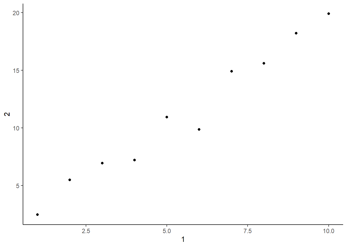

Creating a new column called 3, which is 2 divided by 1.

tibble(
  `1` = 1:10,
  `2` = `1` * 2 + rnorm(length(`1`)),
  `3` = `2` / `1`)

# A tibble: 10 × 3
     `1`    `2`   `3`
   <int>  <dbl> <dbl>
 1     1  0.833 0.833
 2     2  4.02  2.01 
 3     3  5.63  1.88 
 4     4  7.31  1.83 
 5     5 10.6   2.12 
 6     6 11.7   1.95 
 7     7 14.4   2.05 
 8     8 16.0   2.00 
 9     9 18.1   2.01 
10    10 21.9   2.19

Renaming the columns to one, two, and three.

tibble(
  `1` = 1:10,
  `2` = `1` * 2 + rnorm(length(`1`)),
  `3` = `2` / `1`) %>% 
  rename(
    one = `1`,
    two = `2`,
    three = `3`)

# A tibble: 10 × 3
     one   two three
   <int> <dbl> <dbl>
 1     1  2.04  2.04
 2     2  4.10  2.05
 3     3  6.67  2.22
 4     4  7.73  1.93
 5     5 10.1   2.02
 6     6 12.2   2.03
 7     7 13.4   1.91
 8     8 18.3   2.29
 9     9 16.9   1.87
10    10 18.9   1.89